Preparing Meteorological Inputs¶

This section shows a complete example of the current NetCDF-based meteorological workflow in pycequeau.

The workflow assumes that the project already contains a meteo/ERA folder with prepared NetCDF files for the basin.

create the Basin object
derive an additional meteorological variable when needed
load the NetCDF meteorological files
inspect missing values
interpolate the meteorological fields
construct the CEQUEAU meteorological grid
save the resulting NetCDF file

[11]:

import os
import matplotlib.pyplot as plt

from pycequeau.physiographic import Basin
from pycequeau.meteo import MeteoCalculator, NetCDFMeteo
from pycequeau.core.netcdf import intermidiate_interpolation

Expected content of the ERA folder¶

The ERA folder is expected to contain NetCDF files prepared for the basin, usually with one meteorological variable per file. The ERA folder should be located in the following path path/to/your/project/meteo/ERA

The file names themselves do not matter. What matters for pycequeau is that each file contains a supported variable name and valid units metadata.

For the current example project, the files in the folder look like this:

File name	Variable name	Units in this example	Other accepted units
`era5_10m-wind-speed_daily.nc`	`wind`	`m s-1`	`km h-1`
`era5_2m-dewpoint-temperature_daily.nc`	`d2m`	`K`	`C`
`era5_2m-temperature_daily_max.nc`	`tasmax`	`K`	`C`
`era5_2m-temperature_daily_min.nc`	`tasmin`	`K`	`C`
`era5_surface-solar-radiation-downwards_daily.nc`	`ssrd`	`J m-2`	`MJ m-2 d-1MJ m-2J m-2 d-1W m-2`
`era5_surface-thermal-radiation-downwards_daily.nc`	`strd`	`J m-2`	`MJ m-2 d-1MJ m-2J m-2 d-1W m-2`
`era5_total-cloud-cover_daily.nc`	`tcc`	`0-1`	`fraction1%percent`
`era5_total-precipitation_daily.nc`	`tp`	`m`	`mm d-1mmm d-1kg m-2 s-1`
`saturated_vapor_pressure.nc`	`vp`	`mmHg`	`PakPa`

Most of these files come from prepared ERA5 products aggregated to the daily time step. In this workflow, wind speed and vapor pressure are obtained with the meteorological calculators before the complete meteorological dataset is loaded.

In the example below, saturated_vapor_pressure.nc is created from d2m with MeteoCalculator.create_variable_file(...). The wind-speed file follows the same idea, using the meteorological calculators to derive wind from the original wind components. For the calculator API reference, see the meteorological calculators module.

Project configuration¶

Set the project folder, the basin name, and the raster files used to initialize the basin.

[ ]:

project_folder = r"path/to/your/project/"
files_list = ["DEM.tif", # DEM tif file
                "FAC.tif", #Flow accumulation tif file
                "LCF.tif", # Land conver tif file
                "Watershed.tif", # Watershed tif file
                "CAT.tif" #Sub basins tif file
                ]
basin_name = "Margarite"

bassin_versant_file = os.path.join(
    project_folder,
    "results",
    "bassinVersant.mat",
)
meteo_folder = os.path.join(project_folder, "meteo", "ERA")

Create the basin object¶

The basin object is required to project and export the meteorological data to the CEQUEAU grid.

[13]:

basin = Basin(
    project_folder,
    basin_name,
    files_list,
    bassin_versant_file,
)

Plot a sample day¶

A quick plot can be useful to visually inspect a few interpolated meteorological fields before exporting the CEQUEAU file.

[18]:

plot_ds = interpolated.isel(time=0)

fig, axes = plt.subplots(
    ncols=2,
    nrows=2,
    figsize=(12, 10),
)

plot_ds["tMax"].plot(ax=axes[0, 0], cmap="Spectral")
plot_ds["tMin"].plot(ax=axes[0, 1], cmap="Spectral")
plot_ds["rayonnement"].plot(ax=axes[1, 0], cmap="Spectral")
plot_ds["pTot"].plot(ax=axes[1, 1], cmap="Spectral")

axes[0, 0].set_title("tMax")
axes[0, 1].set_title("tMin")
axes[1, 0].set_title("rayonnement")
axes[1, 1].set_title("pTot")

plt.tight_layout()

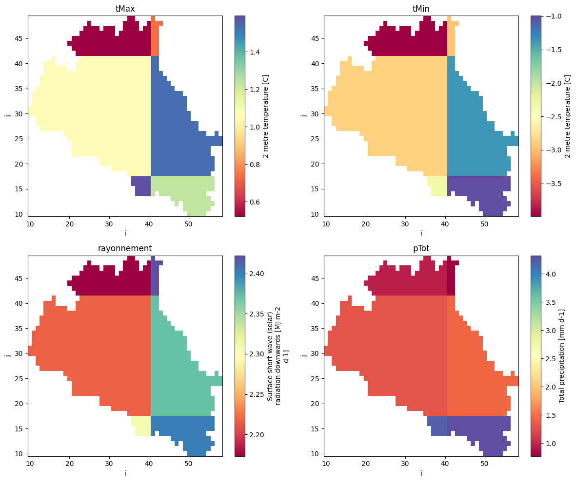
Save the final NetCDF file¶

The resulting CEQUEAU-ready meteorological dataset can then be written to disk.

[19]:

output_file = os.path.join(project_folder, "meteo", "meteo_cequeau.nc")
grid_cequeau.to_netcdf(output_file)
# output_file

Preparing Meteorological Inputs¶

Expected content of the ERA folder¶

Project configuration¶

Create the basin object¶

Load the NetCDF meteorological inputs¶

Downscale the meteorological grid when needed¶

Interpolate the meteorological fields¶

Build the CEQUEAU grid¶

Plot a sample day¶

Save the final NetCDF file¶